

안녕하세요.
오늘은 Amazon 제품 가격 예측 봇 개발의 두 번째 시간입니다.
•
데이터 전처리
•
Baseline 모델 생성
•
LLM 파인튜닝 with GPT
•
LLM 파인튜닝 with LLAMA
이번 세션에서는 LLM 모델을 파인튜닝하기 전에, 기준이 되는 Baseline 모델을 구축하고 평가하도록 하겠습니다.
라이브러리 로드 및 환경 설정
먼저, 이번 시간에 사용할 라이브러리를 로드합니다.
Baseline 모델 구축에 필요한 Scikit-learn 라이브러리와 Gensim 라이브러리를 새롭게 추가했습니다.
import os
import json
import matplotlib.pyplot as plt
import pickle
# More imports for our traditional machine learning
import pandas as pd
import numpy as np
from sklearn.linear_model import LinearRegression
from sklearn.metrics import mean_squared_error, r2_score
from sklearn.preprocessing import StandardScaler
from sklearn.svm import LinearSVR
from sklearn.ensemble import RandomForestRegressor
# And more imports for our NLP related machine learning
from sklearn.feature_extraction.text import CountVectorizer
from gensim.models import Word2Vec
from gensim.utils import simple_preprocess
# Constants - used for printing to stdout in color
GREEN = "\033[92m"
YELLOW = "\033[93m"
RED = "\033[91m"
RESET = "\033[0m"
COLOR_MAP = {"red":RED, "orange": YELLOW, "green": GREEN}
%matplotlib inline
Python
복사
데이터 로드
Baseline 모델 구축을 위해 이전 시간에 전처리 한 제품 데이터를 로드합니다.
제품의 전체 정보를 활용하기 위해, 로컬에 저장한 pickle 데이터를 사용합니다.
# Let's avoid curating all our data again! Load in the pickle files:
with open('train.pkl', 'rb') as file:
train = pickle.load(file)
with open('test.pkl', 'rb') as file:
test = pickle.load(file)
Python
복사
# Remind ourselves the training prompt
print(train[0].prompt)
>> How much does this cost to the nearest dollar?
JS Route 66 Lamp with Shade
The desk lamp base is made of sturdy metal. A metal plate was rolled in to make the body of the lamp base. This durable desk lamp will last for a long time. And its quality is absolutely superb. The desk lamp base is made of sturdy metal Approximately 16 in. H x 10 in. W A metal plate was rolled in to make the body of the lamp base It uses a standard light bulb - A15 LED bulb, which is about 3-inch tall and available at Home Depot, big grocery chains, and online. We DON'T recommend the incandescent bulb due to the excessive heat produced. Please refer to our policy for the product warranty. Style Lamp, Brand JS, Color Silver, Dimensions 10 x 10 x
Price is $46.00
Python
복사
# Remind a test prompt
print(train[0].price)
>> 45.99
Python
복사
Tester 클래스 생성
각 Baseline 모델의 평가를 위한 Tester 클래스를 작성했습니다.
모델의 종류와 무관하게, 동일한 방식으로 예측 결과를 평가하기 위해 하나의 클래스를 정의한 것입니다
class Tester:
def __init__(self, predictor, title=None, data=test, size=250):
self.predictor = predictor
self.data = data
self.title = title or predictor.__name__.replace("_", " ").title()
self.size = size
self.guesses = []
self.truths = []
self.errors = []
self.sles = []
self.colors = []
def color_for(self, error, truth):
if error < 40 or error/truth < 0.2:
return "green"
elif error < 80 or error/truth < 0.4:
return "orange"
else:
return "red"
def run_datapoint(self, i):
datapoint = self.data[i]
guess = self.predictor(datapoint)
truth = datapoint.price
error = abs(guess - truth)
log_error = math.log(truth+1) - math.log(guess+1)
sle = log_error ** 2
color = self.color_for(error, truth)
title = datapoint.title if len(datapoint.title) <= 40 else datapoint.title[:40]+"..."
self.guesses.append(guess)
self.truths.append(truth)
self.errors.append(error)
self.sles.append(sle)
self.colors.append(color)
print(f"{COLOR_MAP[color]}{i+1}: Guess: ${guess:,.2f} Truth: ${truth:,.2f} Error: ${error:,.2f} SLE: {sle:,.2f} Item: {title}{RESET}")
def chart(self, title):
max_error = max(self.errors)
plt.figure(figsize=(12, 8))
max_val = max(max(self.truths), max(self.guesses))
plt.plot([0, max_val], [0, max_val], color='deepskyblue', lw=2, alpha=0.6)
plt.scatter(self.truths, self.guesses, s=3, c=self.colors)
plt.xlabel('Ground Truth')
plt.ylabel('Model Estimate')
plt.xlim(0, max_val)
plt.ylim(0, max_val)
plt.title(title)
plt.show()
def report(self):
average_error = sum(self.errors) / self.size
rmsle = math.sqrt(sum(self.sles) / self.size)
hits = sum(1 for color in self.colors if color=="green")
title = f"{self.title} Error=${average_error:,.2f} RMSLE={rmsle:,.2f} Hits={hits/self.size*100:.1f}%"
self.chart(title)
def run(self):
self.error = 0
for i in range(self.size):
self.run_datapoint(i)
self.report()
@classmethod
def test(cls, function):
cls(function).run()
Python
복사
•
test() 함수를 호출하여, 모델의 예측 성능을 평가합니다. 파라미터인 function은 모델 가격을 예측할 수 있는 기능을 제공해야 합니다. 테스트 데이터에 대한 예측 결과 및 성능을 차트 형태로 제공합니다.
모델 예측 성능
아키텍처(모델) 관점: LLM 모델은 주어진 제품 정보를 입력 받아, 가격을 예측하는 형태입니다. 즉, next token prediction task이며, 예측 가능한 토큰 중 하나를 고르는 것입니다. 따라서, categorical cross entropy 등의 지표를 생각할 수 있습니다.
반면, 전통적 머신러닝 모델의 경우, 회귀 문제로 접근하여 실제 값과 예측 값의 차이를 지표로 삼을 수 있습니다. 해당 프로젝트에서는 MAE(Mean Absolute Error)와 SLE(Squared Log Error)를 사용했습니다.
비즈니스 관점: 모델 종류에 관계 없이, 최대한 정확하게 가격을 예측하여 기여할 수 있는 부분을 생각해야합니다. 예를 들면, 고객의 희망 가격 범위에 맞는 제품을 추천할 수 있습니다. 이때는, 매출 증가량 및 리텐션 등이 비즈니스 지표가 될 수 있겠네요! 본 프로젝트에서는 Hit ratio 를 하나의 지표로 선정하였습니다. Hit ratio의 경우, 예측 오차율이 20% 미만인 예측 횟수를 기반으로 계산하였습니다.
결과적으로, 본 프로젝트에서는 MAE, SLE 및 Hit ratio 세 가지 기준을 통해 각 모델을 평가할 것입니다.
Baseline 모델
Random model
첫 번째 Baseline 모델은 랜덤 모델입니다. 1달러부터 1000달러 중 하나의 가격으로 예측하는 방식입니다.
def random_pricer(item):
return random.randrange(1,1000)
Python
복사
평가의 시간입니다.
# Set the random seed
random.seed(42)
# Run our TestRunner
Tester.test(random_pricer)
>>
1: Guess: $655.00 Truth: $336.28 Error: $318.72 SLE: 0.44 Item: KOHLER K-7401-K-CP Triton Centerset Lava...
2: Guess: $115.00 Truth: $3.22 Error: $111.78 SLE: 10.98 Item: HUYGHAVO Sports Pattern Designed for iPh...
3: Guess: $26.00 Truth: $182.99 Error: $156.99 SLE: 3.68 Item: WERFACTORY Tiffany Floor Lamp Green Stai...
...
248: Guess: $20.00 Truth: $429.00 Error: $409.00 SLE: 9.12 Item: Arotikee Modern Gold Contemporary Crysta...
249: Guess: $115.00 Truth: $1.04 Error: $113.96 SLE: 16.33 Item: Cosmas® 9985SN Satin Nickel Round Cabine...
250: Guess: $952.00 Truth: $13.99 Error: $938.01 SLE: 17.24 Item: welltop Egg Holder for Refrigerator, Lar...
Python
복사
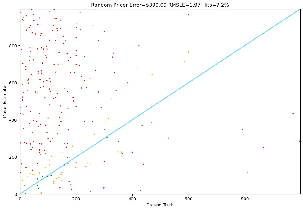
임의로 예측한 만큼, 결과가 안좋네요. 평균적으로 390 달러 만큼 예측을 잘못했고, Hit ratio는 불과 7%입니다.
Linear Regression Model
다음 후보는 선형 회귀 모델입니다!
저는 다음과 같은 피처를 사용하였습니다.
•
weight(제품 중량)
•
rank(제품 랭킹)
•
text_length(제품 설명 문자 길이) → 가공 피처
◦
제품 설명이 풍부할 수록, 보다 정확하게 가격을 예측할 수 있지 않을까 해서 피처로 포함했습니다.
•
is_most_common_40_brands(빈도 수 기반 상위 40위 브랜드 여부) → 가공 피처
•
is_most_common_40_manufacturers(빈도 수 기반 상위 40위 제조사 여부) → 가공 피처
•
is_same_brand_with_manufacturer(제조사 및 브랜드사 일치 여부)
◦
브랜드사에서 직접 제품을 제조할 경우, 부대 비용이 감소할 수 있습니다. 이로 인해, 실제 판매가에 영향을 미칠 수 있습니다.
•
is_discounted(할인 여부)
아래는 각 피처 별 가공(전처리) 함수입니다.
[제품 중량 관련]
# 제품 중량 단위 통일
def get_weight(item):
weight_str = item.features.get('Item Weight')
if weight_str:
parts = weight_str.split(' ')
amount = float(parts[0])
unit = parts[1].lower()
if unit=="pounds":
return amount
elif unit=="ounces":
return amount / 16
elif unit=="grams":
return amount / 453.592
elif unit=="milligrams":
return amount / 453592
elif unit=="kilograms":
return amount / 0.453592
elif unit=="hundredths" and parts[2].lower()=="pounds":
return amount / 100
else:
print(weight_str)
return None
weights = [get_weight(t) for t in train]
weights = [w for w in weights if w]
average_weight = sum(weights)/len(weights)
# 제품 중량 결측치 처리 함수
def get_weight_with_default(item):
weight = get_weight(item)
return weight or average_weight
Python
복사
[제품 랭킹 관련]
# 제품 랭킹 함수
def get_rank(item):
rank_dict = item.features.get("Best Sellers Rank")
if rank_dict:
ranks = rank_dict.values()
return sum(ranks)/len(ranks)
return None
ranks = [get_rank(t) for t in train]
ranks = [r for r in ranks if r]
average_rank = sum(ranks)/len(ranks)
# 제품 랭킹 결측값 처리 함수
def get_rank_with_default(item):
rank = get_rank(item)
return rank or average_rank
Python
복사
# 제품 설명 길이 구하는 함수
def get_text_length(item):
return len(item.test_prompt())
Python
복사
[상위 브랜드 관련]
# investigate the brands
brands = Counter()
for t in train:
brand = t.features.get("Brand")
if brand:
brands[brand]+=1
most_common_40_brands = (info[0] for info in brands.most_common(40))
def is_most_common_40_brands(item):
brand = item.features.get("Brand", None)
if brand is not None:
return brand and brand.lower() in most_common_40_brands
else:
return False
Python
복사
[상위 제조사 관련]
# investigate the manufacturer
manufacturers = Counter()
for t in train:
manufacturer = t.features.get("Manufacturer")
if manufacturer:
manufacturers[manufacturer] += 1
most_common_40_manufacturer = (info[0] for info in manufacturers.most_common(40))
def is_most_common_40_manufacturer(item):
manufacturer = item.features.get("Manufacturer", None)
if manufacturer is not None:
return manufacturer and manufacturer.lower() in most_common_40_manufacturer
else:
return False
Python
복사
[제조사 - 브랜드 사 일치 여부]
def is_same_brand_with_manufacturer(item):
manufacturer = item.features.get("Manufacturer", None)
brand = item.features.get("Brand", "None")
if manufacturer is None or brand is None: return False
else:
if manufacturer == brand: return True
else: return False
Python
복사
[제품 할인 여부]
def is_discounted(item):
discount = item.features.get("Is Discontinued By Manufacturer", None)
if discount is not None and discount == 'Yes': return True
else: return False
Python
복사
[전체 피처 가공 함수]
def get_features(item):
return {
"weight": get_weight_with_default(item),
"rank": get_rank_with_default(item),
"text_length": get_text_length(item),
"is_most_common_40_brands": 1 if is_most_common_40_brands(item) else 0,
"is_most_common_40_manufacturers": 1 if is_most_common_40_manufacturer(item) else 0,
"is_same_brand_with_manufacturer": 1 if is_same_brand_with_manufacturer(item) else 0,
"is_discounted": 1 if is_discounted(item) else 0
}
Python
복사
선형 회귀 모델 학습 및 평가를 위해 데이터를 준비합니다.
# A utility function to convert our features into a pandas dataframe
def list_to_dataframe(items):
features = [get_features(item) for item in items]
df = pd.DataFrame(features)
df['price'] = [item.price for item in items]
return df
train_df = list_to_dataframe(train)
test_df = list_to_dataframe(test)
np.random.seed(42)
# Separate features and target
feature_columns = [
'weight', 'rank', 'text_length',
'is_most_common_40_brands', 'is_most_common_40_manufacturers',
'is_same_brand_with_manufacturer', 'is_discounted'
]
X_train = train_df[feature_columns]
y_train = train_df['price']
X_test = test_df[feature_columns]
y_test = test_df['price']
Python
복사
모델을 학습합니다.
# Train a Linear Regression
model = LinearRegression()
model.fit(X_train, y_train)
Python
복사
Tester 클래스를 통해, 학습된 선형 회귀 모델을 평가합니다.
def linear_regression_pricer(item):
features = get_features(item)
features_df = pd.DataFrame([features])
return model.predict(features_df)[0]
Tester.test(linear_regression_pricer)
>>>
1: Guess: $152.70 Truth: $336.28 Error: $183.58 SLE: 0.62 Item: KOHLER K-7401-K-CP Triton Centerset Lava...
2: Guess: $125.05 Truth: $3.22 Error: $121.83 SLE: 11.54 Item: HUYGHAVO Sports Pattern Designed for iPh...
3: Guess: $158.83 Truth: $182.99 Error: $24.16 SLE: 0.02 Item: WERFACTORY Tiffany Floor Lamp Green Stai...
...
248: Guess: $177.23 Truth: $429.00 Error: $251.77 SLE: 0.78 Item: Arotikee Modern Gold Contemporary Crysta...
249: Guess: $157.33 Truth: $1.04 Error: $156.29 SLE: 18.94 Item: Cosmas® 9985SN Satin Nickel Round Cabine...
250: Guess: $144.20 Truth: $13.99 Error: $130.21 SLE: 5.16 Item: welltop Egg Holder for Refrigerator, Lar...
Python
복사
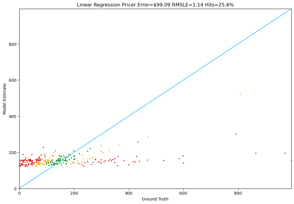
평균 예측 오차 99달러, Hit ratio 25%, SLE는 1.14이네요! 랜덤 모델보다는 훨씬 낫습니다.
Linear Regression Model + Word2Vec
이번에도 동일하게 선형 회귀 모델을 사용합니다.
다만, 입력 피처가 제품 설명입니다!
따라서, 텍스트 데이터를 수치화하는 과정이 필요한 데 이를 위해 Gensim 라이브러리에서 제공하는 Word2Vec을 통해, 임베딩을 수행했습니다.
np.random.seed(42)
# Preprocess the documents
processed_docs = [simple_preprocess(doc) for doc in documents]
# Train Word2Vec model
w2v_model = Word2Vec(sentences=processed_docs, vector_size=400, window=5, min_count=1, workers=8)
def document_vector(doc):
doc_words = simple_preprocess(doc)
word_vectors = [w2v_model.wv[word] for word in doc_words if word in w2v_model.wv]
return np.mean(word_vectors, axis=0) if word_vectors else np.zeros(w2v_model.vector_size)
# Create feature matrix
X_w2v = np.array([document_vector(doc) for doc in documents])
Python
복사
임베딩 피처를 통해, 선형 회귀 모델을 학습하고 평가해봅시다!
# train
word2vec_lr_regressor = LinearRegression()
word2vec_lr_regressor.fit(X_w2v, prices)
# test
Tester.test(word2vec_lr_pricer)
>>>
1: Guess: $167.74 Truth: $336.28 Error: $168.54 SLE: 0.48 Item: KOHLER K-7401-K-CP Triton Centerset Lava...
2: Guess: $0.78 Truth: $3.22 Error: $2.44 SLE: 0.74 Item: HUYGHAVO Sports Pattern Designed for iPh...
3: Guess: $165.31 Truth: $182.99 Error: $17.68 SLE: 0.01 Item: WERFACTORY Tiffany Floor Lamp Green Stai...
...
248: Guess: $274.95 Truth: $429.00 Error: $154.05 SLE: 0.20 Item: Arotikee Modern Gold Contemporary Crysta...
249: Guess: $0.00 Truth: $1.04 Error: $1.04 SLE: 0.51 Item: Cosmas® 9985SN Satin Nickel Round Cabine...
250: Guess: $37.47 Truth: $13.99 Error: $23.48 SLE: 0.89 Item: welltop Egg Holder for Refrigerator, Lar...
Python
복사
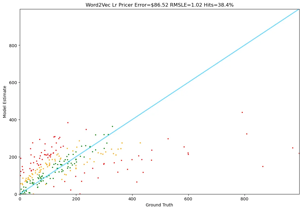
평균 예측 오차 86달러, Hit ratio 38%, SLE는 1.02로서, 기존 선형 회귀 모델의 성능을 뛰어 넘었습니다 :)
Support Vector Machine
다음은 서포트 벡터 기반 회귀 모델입니다.
앞서 Word2Vec 방법론을 통해 생성한 임베딩 피처를 사용하도록 할게요.
np.random.seed(42)
svr_regressor = LinearSVR()
svr_regressor.fit(X_w2v, prices)
Python
복사
이제, 모델을 평가합니다.
def svr_pricer(item):
np.random.seed(42)
doc = item.test_prompt()
doc_vector = document_vector(doc)
return max(float(svr_regressor.predict([doc_vector])[0]),0)
Tester.test(svr_pricer)
>>>
1: Guess: $130.78 Truth: $336.28 Error: $205.50 SLE: 0.88 Item: KOHLER K-7401-K-CP Triton Centerset Lava...
2: Guess: $7.16 Truth: $3.22 Error: $3.94 SLE: 0.43 Item: HUYGHAVO Sports Pattern Designed for iPh...
3: Guess: $164.59 Truth: $182.99 Error: $18.40 SLE: 0.01 Item: WERFACTORY Tiffany Floor Lamp Green Stai...
...
248: Guess: $203.40 Truth: $429.00 Error: $225.60 SLE: 0.55 Item: Arotikee Modern Gold Contemporary Crysta...
249: Guess: $0.00 Truth: $1.04 Error: $1.04 SLE: 0.51 Item: Cosmas® 9985SN Satin Nickel Round Cabine...
250: Guess: $45.09 Truth: $13.99 Error: $31.10 SLE: 1.26 Item: welltop Egg Holder for Refrigerator, Lar...
Python
복사
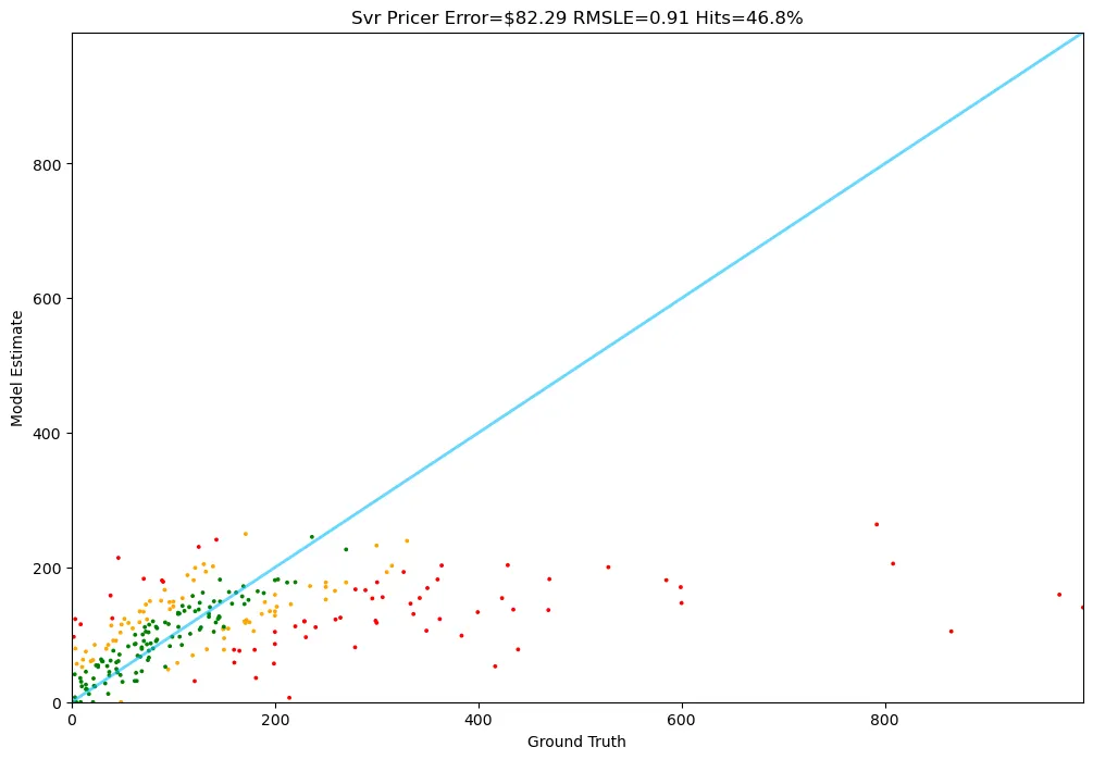
평균 예측 오차 82달러, Hit ratio 46%, SLE는 0.91로서, 모든 Baseline 모델 중 가장 높은 성능을 보이네요!
정리
이번 시간에는, LLM 모델을 파인튜닝 하기에 앞서, 기준이 되는 네 가지 Baseline 모델을 학습하고 평가하였습니다.
Baseline 모델 목록 | 평균 예측 오차(MAE, $) | SLE | Hit ratio(%) |
Random Model | 390.09 | 1.97 | 7.2 |
Linear Regression Model | 99.09 | 1.14 | 25.6 |
Linear Regression + Word2Vec | 86.52 | 1.02 | 38.4 |
Support Vector Machine | 82.29 | 0.91 | 46.8 |
GPT-4o-Mini with Fine-tuning | |||
Meta-Llama-3.1-8B with Fine-tuning |
다음 포스팅에서는 Closed-source 모델을 대표하는 GPT-4와 Open-source 모델의 대표 격인 Llama-3.1-8B 모델을 파인튜닝하고, 성능 표의 빈 값을 채워보겠습니다!!
파인튜닝한 모델의 성능이 개선 되었을까요? 그렇다면, 얼마나 개선되었을까요? 최고의 모델은 과연 누가 될까요?
궁금해 미치겠군요 ㅎㅎㅎ